| Other version | Source | Contact
Autovar
Select .sav, .dta, or .csv file containing the data set.

Run Download Results View syntax help Fig. height Fig. width

About

Autovar can be used to find VAR models for time series data. Its main functionality is producing a list of VAR models that do not invalidate the model assumptions. Autovar can summarize over the models to provide insight into, e.g., significant contemporaneous correlation and Granger causalities present in the data set.

While Autovar is available as an R package, part of its functionality is exposed through this web application, running some of the exported Autovar functions (depending on the options selected) and showing the results.

Example data sets and use

To reproduce the results from one of the data sets used in our IEEE JBHI paper, please download the Dataset45Jdaggem.dta data set file. Load the file in Autovar by clicking "Browse" or "Choose file" above. The user interface will then change as it reads the columns from the data set. Set it to select the "Stre" and "Musc" columns as shown below.

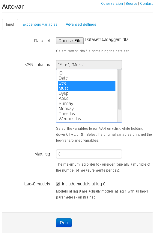
Here, we opt to include lag 0 models as well by ticking the box.

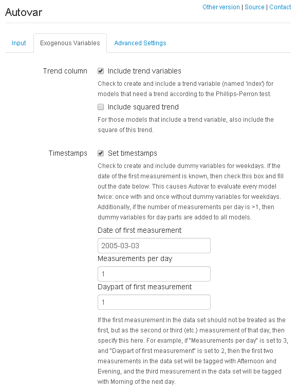
Optionally, we can provide Autovar with some more information about the data set. For example, if we know that this data set describes a study with a single measurement per day, and the first measurement was completed on the 3rd of March, we can specify this as shown in the image below. Setting timestamps enables Autovar to generate and possibly include dummy variables for days and day parts in its models, to account for cyclity if needed.

Finally, check "Sort output using BIC instead of AIC" for "Model evaluation" on the "Advanced Settings" tab (not shown). Pressing "Run" will then show the output of running a sequence of functions(*) exported by the Autovar package. If all went correctly, the tab on the right should show as part of its output the following:

The valid models (sorted by BIC score):
A: (AIC: 1253.375 (orig: 277.265), BIC: 1274.814 (orig: 298.704)) : Musc ~Granger causes~ Stre (0.00332); Stre -Granger causes- Musc (0.000955)

followed by the model details. Note that the listed 1274.814 BIC score corresponds to the number displayed in the row for "45 Stre Musc" in Table I of our IEEE JBHI paper as the BIC score of the best model found by Autovar.

  • Another data set is presented in aug_pp5_da.sav. This data set works with all settings at default. Simply click "Choose file" to select the data set, select "Activity" and "Depression" as VAR columns, and press "Run."
  • Also available is the data set Dataset57Sdaggem.dta. For this data set, use the same settings as for Dataset47Jdaggem.dta described above, but for the Stre Bowe combination, specify max. lag 7 on the input tab and check "Exclude more outliers" on the advanced settings tab.

(*) To reproduce these results using the R package rather than this web app, note that for the given settings, Autovar loads the data set using load_file, adds a trend column using add_trend, adds day dummy columns using set_timestamps, plots the variables using visualize (not required), and then looks for var models and summarize over then by calling var_main, contemporaneous_correlations_plot, var_summary, and print_best_models. The source code for all these functions is publicly available on GitHub. For syntax help on all exported functions, please see the docs section.

Select the variables to run VAR on (click while holding down CTRL or ⌘). Select the original variables only, not the log-transformed variables.
The maximum lag order to consider (typically a multiple of the number of measurements per day).
Models at lag 0 are actually models at lag 1 with all lag-1 parameters constrained.
Check to create and include a trend variable (named 'index') for models that need a trend according to the Phillips-Perron test. For those models that include a trend variable, also include the square of this trend.
Check to create and include dummy variables for weekdays. If the date of the first measurement is known, then check this box and fill out the date below. This causes Autovar to evaluate every model twice: once with and once without dummy variables for weekdays. Additionally, if the number of measurements per day is >1, then dummy variables for day parts are added to all models. If the first measurement in the data set should not be treated as the first, but as the second or third (etc.) measurement of that day, then specify this here. For example, if "Measurements per day" is set to 3, and "Daypart of first measurement" is set to 2, then the first two measurements in the data set will be tagged with Afternoon and Evening, and the third measurement in the data set will be tagged with Morning of the next day.
Select the column names to include as exogenous variables (click while holding down CTRL or ⌘). Do not select trend variables, weekday dummies, or day part dummies here: use the options above instead. Furthermore, in most cases it's not needed to select outlier columns here either since Autovar generates and uses its own. Thus, only select columns here that provide additional contextual information that cannot be derived from the VAR columns. For example, days during which a patient was working.
Use only when you find no models. Enabling this option will find more models but they exclude more data in 'outlier' dummy variables.
To determine whether each outlier should have its own exogenous variable. This will make a difference only when there is a variable with multiple outliers.
When checked, Skewness and Kurtosis testing is performed using the Jarque-Bera test instead of the sktest. The Jarque-Bera test is sometimes more strict but potentially incorrect.
When checked, a simpler method for finding restrictions is used (no extensive search, no checking of model validity per step).
Use only when you have a large (>=4) number of variables and when using Autovar normally runs for more than 10 minutes. Enabling this option will override some settings to make Autovar run faster, but return fewer/worse models.
When checked, models are assessed by their BIC score instead of their AIC score. This affects the order in which the accepted models are printed and the way in which restrictions are set on the constrained models.
When checked, the system will completely ignore Granger causalities with p-values between 0.05 and 0.10
When checked, all constraints and exogenous variables are always shown (i.e., it will now show exogenous variables that were included but constrained in all equations), and the constraints are formatted like in Stata.